Tidy Tuesday: Mario Kart World Record
I’m finally venturing into the world of Tidy Tuesday. This week is all about Mario Kart.
The Data
The data this week comes from Mario Kart World Records and contains world records for the classic (if you’re a 90’s kid) racing game on the Nintendo 64.
This Video talks about the history of Mario Kart 64 World Records in greater detail. Despite it’s release back in 1996 (1997 in Europe and North America), it is still actiely played by many and new world records are achieved every month.
The game consists of 16 individual tracks and world records can be achieved for the fastest single lap or the fastest completed race (three laps). Also, through the years, players discovered shortcuts in many of the tracks. Fortunately, shortcut and non-shortcut world records are listed separately.
Furthermore, the Nintendo 64 was released for NTSC- and PAL-systems. On PAL-systems, the game runs a little slower. All times in this dataset are PAL-times, but they can be converted back to NTSC-times.
Import data
Read in with tidytuesdayR package. This loads the readme and all the datasets for the week of interest.
library(tidyverse)
# install.packages("tidytuesdayR")
tuesdata <- tidytuesdayR::tt_load('2021-05-25')##
## Downloading file 1 of 2: `drivers.csv`
## Downloading file 2 of 2: `records.csv`records <- tuesdata$records
drivers <- tuesdata$driversLook at the data
str(records)## spec_tbl_df [2,334 x 9] (S3: spec_tbl_df/tbl_df/tbl/data.frame)
## $ track : chr [1:2334] "Luigi Raceway" "Luigi Raceway" "Luigi Raceway" "Luigi Raceway" ...
## $ type : chr [1:2334] "Three Lap" "Three Lap" "Three Lap" "Three Lap" ...
## $ shortcut : chr [1:2334] "No" "No" "No" "No" ...
## $ player : chr [1:2334] "Salam" "Booth" "Salam" "Salam" ...
## $ system_played : chr [1:2334] "NTSC" "NTSC" "NTSC" "NTSC" ...
## $ date : Date[1:2334], format: "1997-02-15" "1997-02-16" ...
## $ time_period : chr [1:2334] "2M 12.99S" "2M 9.99S" "2M 8.99S" "2M 6.99S" ...
## $ time : num [1:2334] 133 130 129 127 125 ...
## $ record_duration: num [1:2334] 1 0 12 7 54 0 0 27 0 64 ...
## - attr(*, "spec")=
## .. cols(
## .. track = col_character(),
## .. type = col_character(),
## .. shortcut = col_character(),
## .. player = col_character(),
## .. system_played = col_character(),
## .. date = col_date(format = ""),
## .. time_period = col_character(),
## .. time = col_double(),
## .. record_duration = col_double()
## .. )Variables of interest for me are time which is in seconds, and probably type for the type of track, and shortcut because times will be different if the player used a shortcut.
Question to explore: Which track is the fastest?
Start by looking at a distribution of record times totally overall.
ggplot(records, aes(x=time)) + geom_histogram()## `stat_bin()` using `bins = 30`. Pick better value with `binwidth`.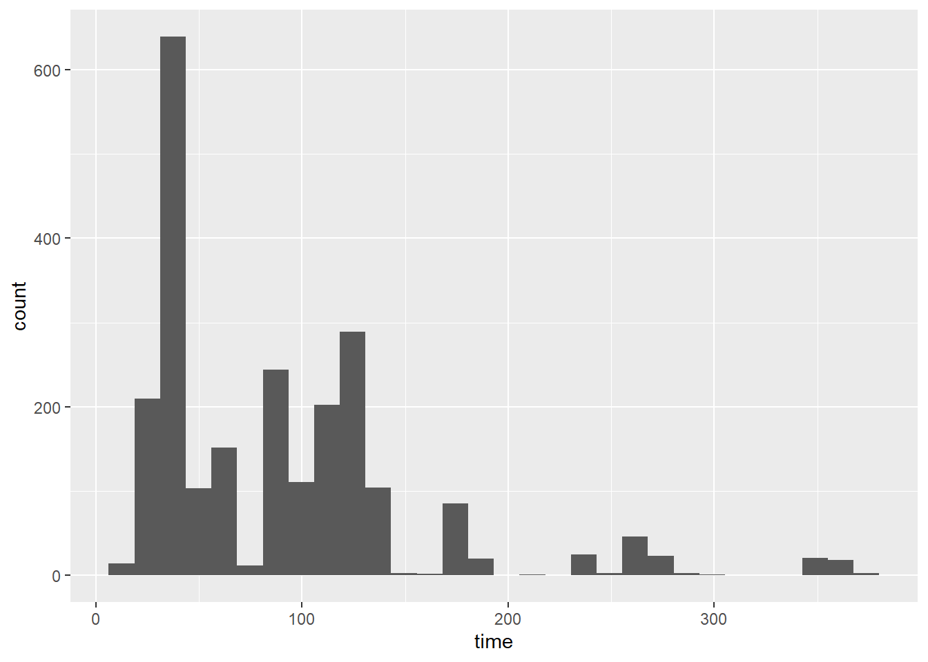
Skewed right.. large peak around 45s ish. Makes me wonder if there is one track that is played more often. I bet the different time “groups” are due to different tracks.
How many tracks are there?
table(records$track)##
## Banshee Boardwalk Bowser's Castle Choco Mountain
## 83 69 148
## D.K.'s Jungle Parkway Frappe Snowland Kalimari Desert
## 180 180 169
## Koopa Troopa Beach Luigi Raceway Mario Raceway
## 89 147 160
## Moo Moo Farm Rainbow Road Royal Raceway
## 81 179 149
## Sherbet Land Toad's Turnpike Wario Stadium
## 143 196 201
## Yoshi Valley
## 16016 - not too many.. Banshee Boardwalk and Bowser’s Castle don’t seem to be played much because they don’t have a lot of records. Or perhaps one person dominated the record board and noone can beat them. Not a high turnover world record.
ggplot(records, aes(x=time)) +
  geom_histogram() +
  facet_wrap(~track)
## `stat_bin()` using `bins = 30`. Pick better value with `binwidth`.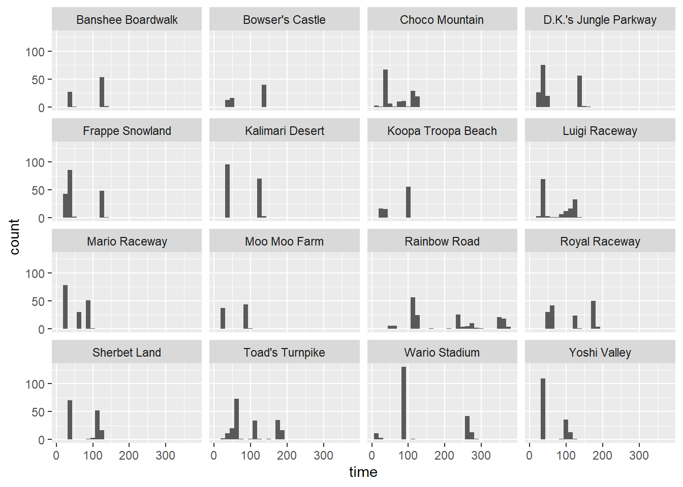
Rainbow Road has the highest variability in record times. Three peaks, probably something to do with track type or shortcuts.
Going back to the original question, which track is the fastest, let’s just grab the minimum record time. Find the row with the minimum time.
records[which(records$time == min(records$time)),]## # A tibble: 1 x 9
## track type shortcut player system_played date time_period time
## <chr> <chr> <chr> <chr> <chr> <date> <chr> <dbl>
## 1 Wario Stad~ Three ~ Yes VAJ NTSC 2020-07-30 14.59S 14.6
## # ... with 1 more variable: record_duration <dbl>That was a base R solution. Here is a ‘tidyverse’ solution.
records %>%
  arrange(time) %>%
slice(1)## # A tibble: 1 x 9
## track type shortcut player system_played date time_period time
## <chr> <chr> <chr> <chr> <chr> <date> <chr> <dbl>
## 1 Wario Stad~ Three ~ Yes VAJ NTSC 2020-07-30 14.59S 14.6
## # ... with 1 more variable: record_duration <dbl>The fastest track time was on Wario Stadium, using a shortcut.
Side tangent
What is the time distribution separated by shortcut?
ggplot(records, aes(y=time, x=shortcut, fill = shortcut)) +
  geom_boxplot() +
  facet_wrap(~track)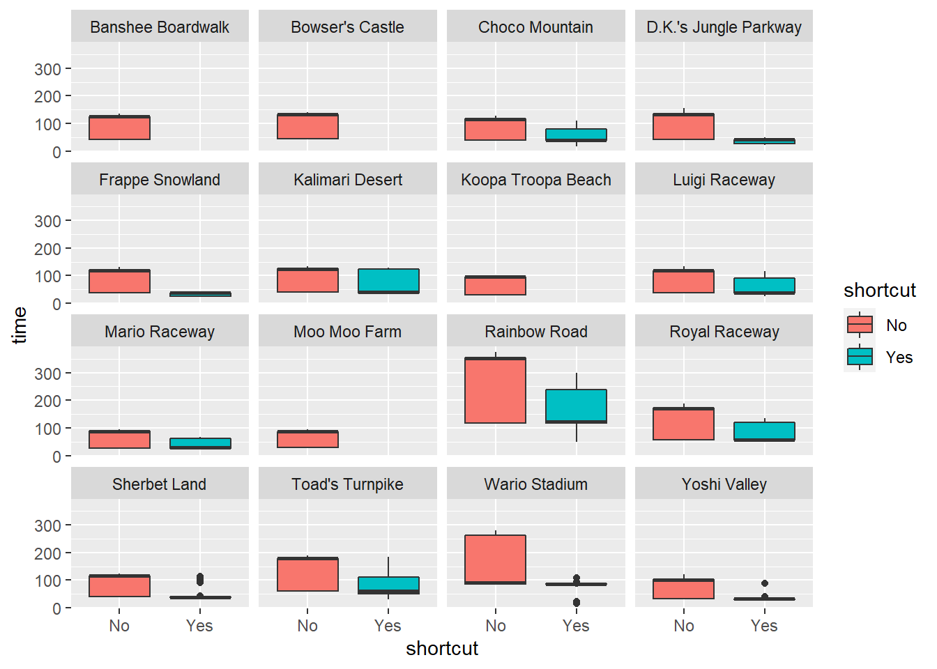
Shortcut doesn’t help Kalimari Desert…spread. The median is very different. Let’s look one more time at distribution, but switch to density so we can see overlap.
ggplot(records, aes(x=time, color = shortcut)) +
  geom_density() +
  facet_wrap(~track, scales = "free")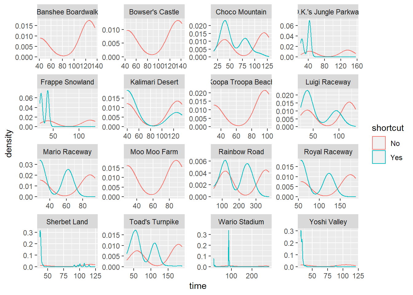
This also shows us that shortcuts were discovered on all tracks except:
- Banshee Boardwalk
- Bowser’s Castle
- Koopa Troopa Beach
- Moo Moo Farm
How does tracks relate to players? Do players have favorite tracks?
How many players?
length(unique(records$player))## [1] 65Lets look at players with only a certain amount of world records.
records %>%
  group_by(player) %>%
  summarise(n=n()) %>%
  arrange(desc(n)) %>%
  ggplot(aes(x=n)) + geom_histogram()
## `stat_bin()` using `bins = 30`. Pick better value with `binwidth`.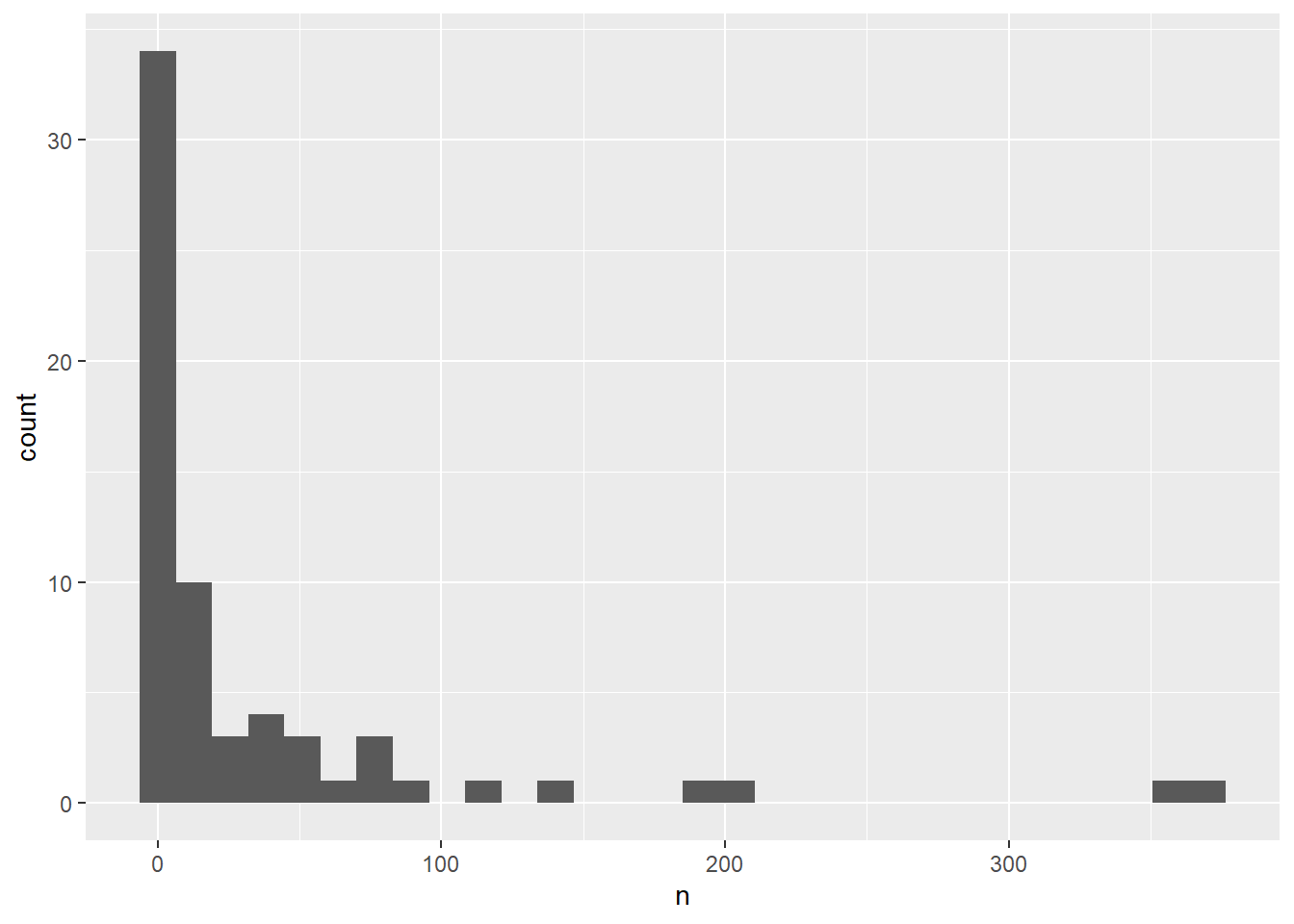
Let’s only look at the players with more than 100 world records. The ELITE!
top.players <- records %>%
  group_by(player) %>%
  summarise(n=n()) %>%
  filter(n>100)

top.players## # A tibble: 6 x 2
## player n
## <chr> <int>
## 1 abney317 118
## 2 Booth 141
## 3 Dan 201
## 4 MJ 197
## 5 MR 351
## 6 Penev 371We have 6 players. Let’s get their track data.
top.player.tracks <- top.players %>%
  left_join(records)
## Joining, by = "player"head(top.player.tracks)## # A tibble: 6 x 10
## player n track type shortcut system_played date time_period time
## <chr> <int> <chr> <chr> <chr> <chr> <date> <chr> <dbl>
## 1 abney3~ 118 Luigi~ Thre~ Yes NTSC 2016-03-22 1M 29.94S 89.9
## 2 abney3~ 118 Luigi~ Thre~ Yes NTSC 2016-03-24 1M 27.45S 87.4
## 3 abney3~ 118 Luigi~ Thre~ Yes NTSC 2021-02-09 44.97S 45.0
## 4 abney3~ 118 Luigi~ Thre~ Yes NTSC 2021-02-09 44.45S 44.4
## 5 abney3~ 118 Luigi~ Thre~ Yes NTSC 2021-02-09 42.47S 42.5
## 6 abney3~ 118 Luigi~ Thre~ Yes NTSC 2021-02-09 39.05S 39.0
## # ... with 1 more variable: record_duration <dbl>Did they all use shortcuts?
table(top.player.tracks$shortcut)##
## No Yes
## 912 467no! Did they all use the same system?
table(top.player.tracks$system_played)##
## NTSC PAL
## 198 1181Look at distribution of track times by track and player
ggplot(top.player.tracks, aes(x=time, color=shortcut)) +
  geom_density() +
facet_grid(track ~ player, scales="free")## Warning: Groups with fewer than two data points have been dropped.
## Warning: Groups with fewer than two data points have been dropped.
## Warning: Groups with fewer than two data points have been dropped.
## Warning: Groups with fewer than two data points have been dropped.
## Warning: Groups with fewer than two data points have been dropped.
## Warning: Groups with fewer than two data points have been dropped.
## Warning: Groups with fewer than two data points have been dropped.
## Warning: Groups with fewer than two data points have been dropped.
## Warning: Groups with fewer than two data points have been dropped.
## Warning: Groups with fewer than two data points have been dropped.
## Warning: Groups with fewer than two data points have been dropped.
## Warning: Groups with fewer than two data points have been dropped.
## Warning: Groups with fewer than two data points have been dropped.
## Warning: Groups with fewer than two data points have been dropped.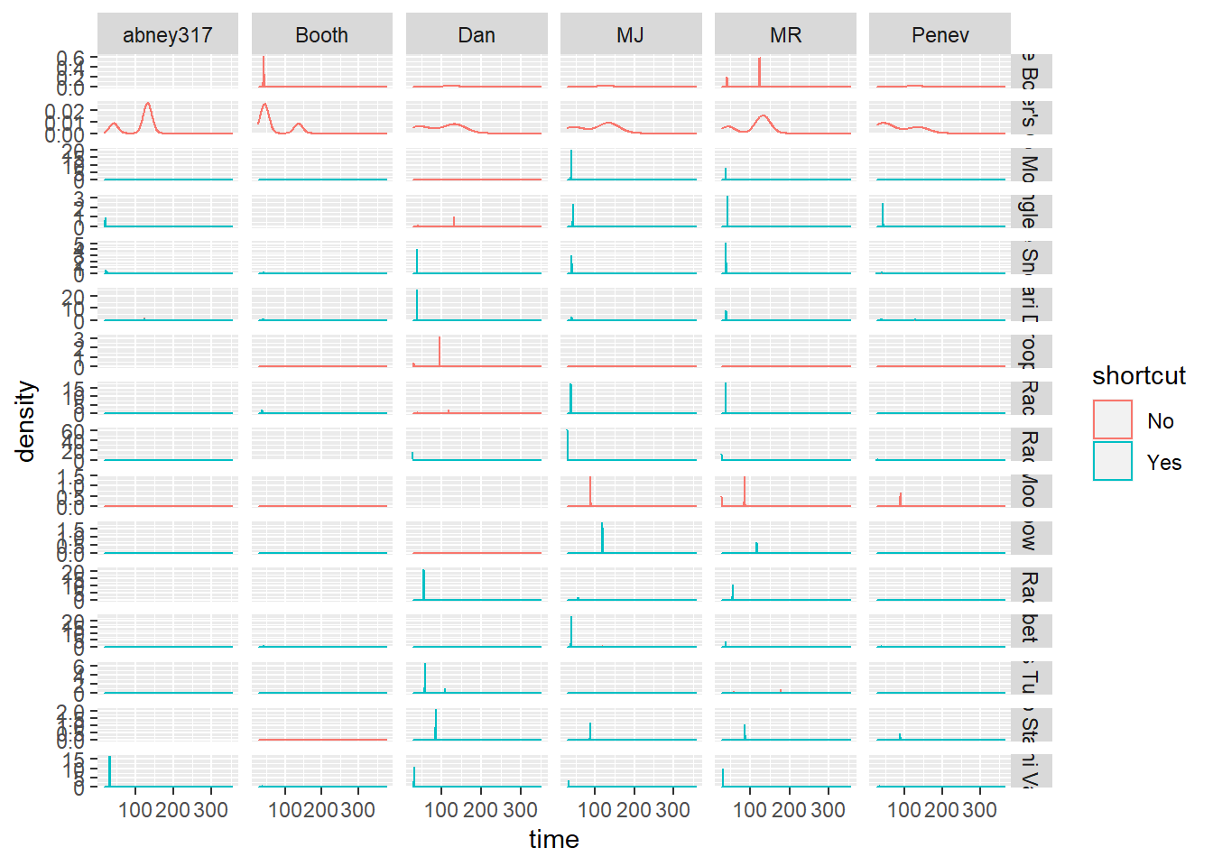
Hard to read, let’s change to one line per player.
ggplot(top.player.tracks, aes(x=time, color=player)) +
  geom_density() +
facet_grid(track ~ shortcut, scales="free")## Warning: Groups with fewer than two data points have been dropped.
## Warning: Groups with fewer than two data points have been dropped.
## Warning: Groups with fewer than two data points have been dropped.
## Warning: Groups with fewer than two data points have been dropped.
## Warning: Groups with fewer than two data points have been dropped.
## Warning: Groups with fewer than two data points have been dropped.
## Warning: Groups with fewer than two data points have been dropped.
## Warning: Groups with fewer than two data points have been dropped.
## Warning: Groups with fewer than two data points have been dropped.
## Warning: Groups with fewer than two data points have been dropped.
## Warning: Groups with fewer than two data points have been dropped.
## Warning: Groups with fewer than two data points have been dropped.
## Warning: Groups with fewer than two data points have been dropped.
## Warning: Groups with fewer than two data points have been dropped.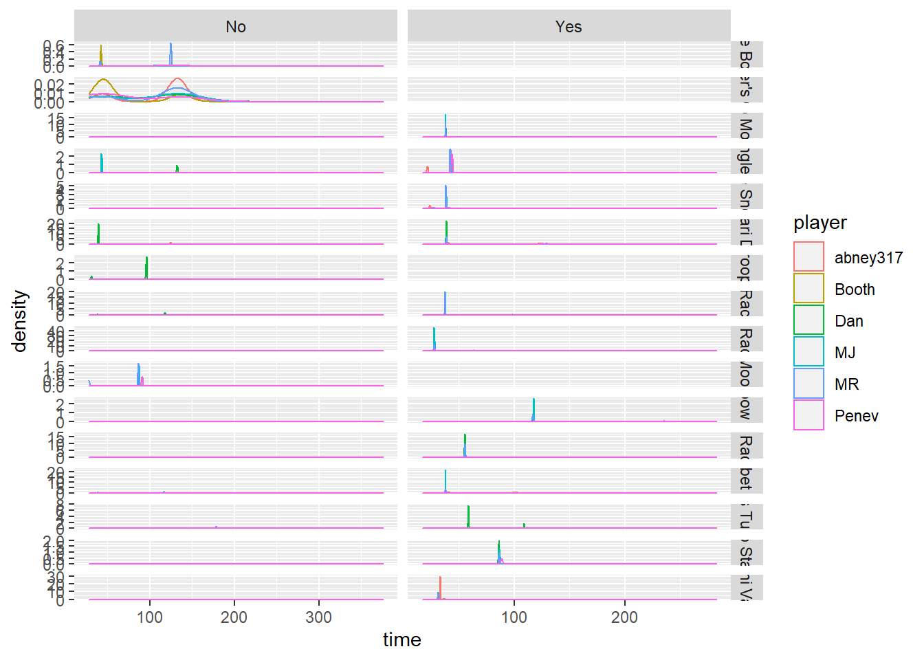
Look at shortcuts vs not totally separately so that the panels can wrap and be more visible. Especially for Penev. I can’t see what they’re doing at all.
top.player.tracks %>%
  filter(shortcut == "No") %>%
  ggplot(aes(x=time, color=player)) +
    geom_density() +
facet_wrap(~track, scales="free")## Warning: Groups with fewer than two data points have been dropped.
## Warning: Groups with fewer than two data points have been dropped.
## Warning: Groups with fewer than two data points have been dropped.
## Warning: Groups with fewer than two data points have been dropped.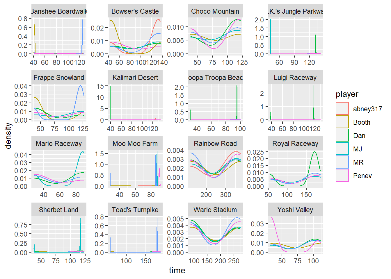
Things I noticed:
- There’s still two peaks for most maps, even though we’re looking at records that were won not using a shortcut. So there is something else going on that affects track time.
- PENEV dominated Yoshi Valley
- Only MR and PENEV play Toad’s Turnpike
- There are 7 maps or so that don’t have high turnover with records.
look closer at Banshee Boardwalk
top.player.tracks %>%
  filter(shortcut == "No",
         track == "Banshee Boardwalk") %>%
  ggplot(aes(x=type, y=time, color=player)) +
  geom_point()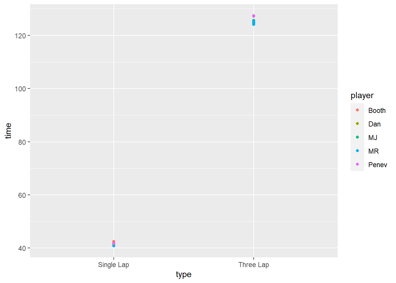
That’s exactly what was driving the two distinct peaks for most if not all maps. That’s something we should have taken into consideration earlier on.